A quick Jupyter notebook about LSTMs and Copulas using tensorflow probability.
Introduction
As commonly known, LSTMs (Long short-term memory networks) are great for dealing with sequential data. One such example are multivariate time-series data. Here, LSTMs can model conditional distributions for complex forecasting problems.
For example, consider the following conditional forecasting distribution:
![\[\begin{gathered} p\left(y_{t+1} \mid y_t\right)=\mathcal{N}\left(y_{t+1} \mid \mu_\theta\left(y_t\right), \Sigma_\theta\left(y_t\right)\right) \\ \mu_\theta\left(y_t\right)=f\left(y_t, h_t\right)_\mu \\ \Sigma_\theta\left(y_t\right)=L_\theta\left(y_t\right) L_\theta\left(y_t\right) \\ L_\theta\left(y_t\right)=f\left(y_t, h_t\right)_L \end{gathered}\]](https://sarem-seitz.com/wp-content/ql-cache/quicklatex.com-d4f361db8a3fb6279d432c8593ff8992_l3.png "Rendered by QuickLaTeX.com")
 LSTM mean output given hidden state
 LSTM covariance cholesky output given hidden state
Notice that we predict the cholesky decomposition of the conditional covariance matrix. This ensures that the resulting covariance matrix is positive semi-definite. Now, this approach would allow us to model quite complex dynamical problems.
On the other hand, however, the degrees of freedom in this model will rapidly explode with increasing dimensionality D of the multivariate time-series. After all, we need (D^2+D)/2 LSTM outputs for the covariance structure alone. This can clearly lead to overfitting quite easily.
Another disadvantage is the assumption of a conditionally Gaussian time-series. As soon as our time-series is not a vector of real-numbers, this model does not work anymore.
Thus, a potential solution should satisfy two properties:
- Allow to parsimoniously handle high-dimensional time-series
- Work with conditionally non-Gaussian time-series
LSTMs with Gaussian Copula
As a potential solution, we could separate the dependency among the time-series from their marginal distribution. Hence, let us presume constant conditional dependency between the time-series but varying conditional marginals. This indicates that a Copula model might be a good approach – for simplicity, we use a Gaussian Copula.
Since the basics of the Gaussian Copula have been discussed in this previous article, we won’t repeat them here.
In summary, our model looks as follows:
![\[p\left(y_{t+1} \mid y_t\right)=\prod_{d=1}^D p_d\left(y_{t+1}^{(d)} \mid \theta_d\left(y_t\right)\right) \cdot c\left(F\left(y_{t+1}^{(1)} \mid \theta_1\left(y_t\right)\right), \ldots, F\left(y_{t+1}^{(D)} \mid \theta_D\left(y_t\right)\right) ; R\right)\]](https://sarem-seitz.com/wp-content/ql-cache/quicklatex.com-2bc97191182433ca88e4c402da35aaa7_l3.png "Rendered by QuickLaTeX.com")
 -th marginal forecast density of
  -th time-series
 -th conditional parameter vector modelled as the output of the LSTM
 Gaussian Copula density with dependency parameter matrix
 d-th marginal forecast c.d.f.
This allows us to deal with arbitrary continuous marginal distributions. In fact, we could even work with mixed continuous marginal distributions. In order to achieve sparsity in the copula parameter matrix, we could, for example, add a regularization term as is typically done when estimating high-dimensional covariance matrices.
The only drawback now is the assumption of a constant dependency over time. If this contradicts the data at hand, we might need to model the copula parameter in an auto-regressive manner as well. A low-rank matrix approach could preserve some parsimony then.
To show how this could be implemented in the case of Gaussian marginals, I have created a quick Jupyter notebook with tensorflow. Regarding the Copula part, the tensorflow example on Gaussian Copulas has a ready-made implementation using tensorflow probability bijectors.
Implementation (sketch, not too much explanation from here on)
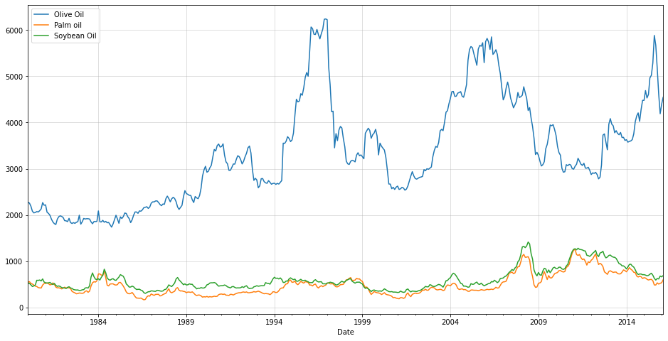
Data taken from https://www.kaggle.com/datasets/vagifa/usa-commodity-prices. We will use only culinary oil price, presuming that there is some underlying correlation among them.
import pandas as pd
import matplotlib.pyplot as plt

df = pd.read_csv("../data/commodity-prices-2016.csv")
df = df.set_index("Date")
df.index = pd.to_datetime(df.index)

oils = df[["Olive Oil","Palm oil","Soybean Oil"]]

oils.plot(figsize=(16,8))
plt.grid(alpha=0.5)


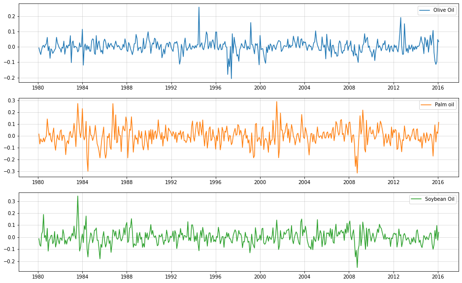
Use log-difference prices for standardization
(i.e. ‘log-returns’)
import numpy as np

oils_ld = np.log(oils).diff().iloc[1:,:]

fig, ax = plt.subplots(3,1, figsize = (16,10))
ax[0].plot(oils_ld["Olive Oil"],label="Olive Oil",color="C0")
ax[1].plot(oils_ld["Palm oil"], label="Palm oil",color="C1")
ax[2].plot(oils_ld["Soybean Oil"], label="Soybean Oil",color="C2")
[a.grid(alpha=0.5) for a in ax]
[a.legend() for a in ax]
Create lag-1 features as input
We might want to go to higher lags for increased accuracy.
oils_lagged = pd.concat([oils_ld.shift(1),oils_ld],axis=1).iloc[1:,:]
oils_lagged.columns = [c+"_l1" for c in oils_ld.columns] + list(oils_ld.columns)

X_train = oils_lagged.iloc[:-12,:3].values
y_train = oils_lagged.iloc[:-12,3:].values
X_test = oils_lagged.iloc[-12:,:3].values
y_test = oils_lagged.iloc[-12:,3:].values
Create the model
(see here for further reference)
import tensorflow as tf
from tensorflow import keras
from tensorflow.keras import layers
import tensorflow_probability as tfp
tfd = tfp.distributions
tfb = tfp.bijectors

class GaussianCopulaTriL(tfd.TransformedDistribution):
    def __init__(self, loc, scale_tril):
        super(GaussianCopulaTriL, self).__init__(
            distribution=tfd.MultivariateNormalTriL(
                loc=loc,
                scale_tril=scale_tril),
            bijector=tfb.NormalCDF(),
            validate_args=True,
            name="GaussianCopulaTriLUniform")


class CopulaLSTMModel(tf.keras.Model):

    def __init__(self, input_dims=3, output_dims=3):
        super().__init__()
        self.input_dims = input_dims
        self.output_dims = output_dims

        #use LSTM state to ease training and testing state transition
        self.c0 = tf.Variable(tf.ones([1,input_dims]), trainable = True)
        self.h0 = tf.Variable(tf.ones([1,input_dims]), trainable = True)

        self.lstm = layers.LSTM(input_dims,
                                         batch_size=(1,1,input_dims),
                                         return_sequences=True,
                                         return_state=True
                                        )

        self.mean_layer = layers.Dense(output_dims)
        self.std_layer = layers.Dense(output_dims,activation=tf.nn.softplus)

        self.chol = tf.Variable(tf.random.normal((output_dims,output_dims)), trainable = True)


    def call(self, inputs):
        lstm_out = self.lstm(inputs, initial_state = [self.c0, self.h0])[0]
        means = self.mean_layer(lstm_out)
        stds = self.std_layer(lstm_out)

        distributions = tfd.Normal(means, stds)

        return distributions


    def call_with_state(self, inputs, c_state, h_state):
        #explicitly use and return the initial state - primarily for forecasting
        lstm_out, c_out, h_out = self.lstm(inputs, initial_state = [c_state, h_state])


        means = self.mean_layer(lstm_out)
        stds = self.std_layer(lstm_out)

        distributions = tfd.Normal(means, stds)

        return distributions, c_out, h_out


    def get_normalized_covariance(self):
        unnormalized_covariance = self.chol@tf.transpose(self.chol)
        normalizer = tf.eye(self.output_dims) * 1./(tf.linalg.tensor_diag_part(unnormalized_covariance)**0.5)

        return normalizer@unnormalized_covariance@normalizer


    def conditional_log_prob(self, inputs, targets):
        marginals = self.call(inputs)
        marginal_lpdfs = tf.reshape(marginals.log_prob(targets),(-1,self.output_dims))

        copula_transformed = marginals.cdf(y_train)
        normalized_covariance = self.get_normalized_covariance()  #need covariance matrix with unit diagonal for Gaussian Copula
        copula_dist = GaussianCopulaTriL(loc=tf.zeros(self.output_dims),scale_tril = tf.linalg.cholesky(normalized_covariance))

        copula_lpdfs = copula_dist.log_prob(copula_transformed)

        return tf.reduce_mean(tf.math.reduce_sum(marginal_lpdfs,1) + copula_lpdfs)


    def train_step(self, data):
        #custom training steps due to custom loglikelihood-loss
        x, y = data

        with tf.GradientTape() as tape:
            loss = -self.conditional_log_prob(x,y)

        trainable_vars = self.trainable_weights + self.lstm.trainable_weights + self.mean_layer.trainable_weights + self.std_layer.trainable_weights
        gradients = tape.gradient(loss, trainable_vars)

        self.optimizer.apply_gradients(zip(gradients, trainable_vars))

        return {"Current loss": loss}


    def sample_forecast(self, X_train, y_train, forecast_periods = 12):
        #this is still quite slow; should be optimized if used for a real-world problem

        normalized_covariance = self.get_normalized_covariance()
        copula_dist = tfp.distributions.MultivariateNormalTriL(scale_tril = tf.linalg.cholesky(normalized_covariance))
        copula_sample = tfp.distributions.Normal(0,1).cdf(copula_dist.sample(forecast_periods))

        sample = []

        input_current = y_train

        for t in range(forecast_periods):

            _, c_current, h_current = self.lstm(X_train)

            new_dist, c_current, h_current = self.call_with_state(tf.reshape(input_current,(1,1,self.input_dims)), c_current, h_current)

            input_current = new_dist.quantile(tf.reshape(copula_sample[t,:],(1,1,self.output_dims)))
            sample.append(tf.reshape(input_current,(1,self.output_dims)).numpy().reshape(1,self.output_dims))

        return np.concatenate(sample)
Train the model
np.random.seed(123)
tf.random.set_seed(123)

test = CopulaLSTMModel()

test.compile(optimizer="adam")

test.fit(X_train.reshape(1,-1,3),y_train.reshape(1,-1,3), epochs = 250, verbose=0) #relatively fast
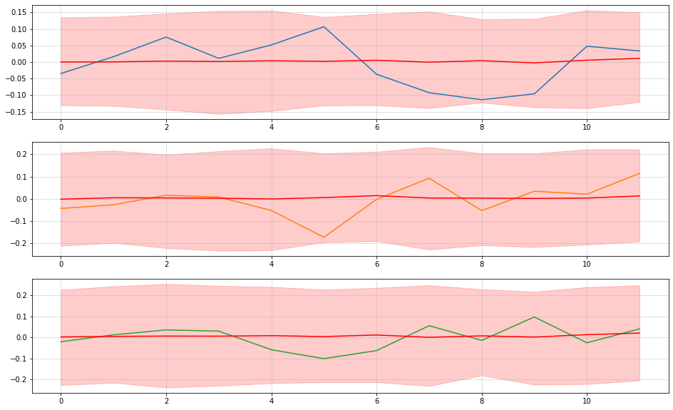
Raw log-diff predictions
np.random.seed(123)
tf.random.set_seed(123)

samples = [test.sample_forecast(X_train.reshape(1,-1,3),y_train[-1,:].reshape(1,1,3)) for _ in range(500)] #very slow, grab a coffee or two

samples_restructured = [np.concatenate(list(map(lambda x: x[:,i].reshape(-1,1),samples)),1) for i in range(3)]
means = [np.mean(s,1) for s in samples_restructured]
lowers = [np.quantile(s,0.05,1) for s in samples_restructured]
uppers = [np.quantile(s,0.95,1) for s in samples_restructured]

fig, ax = plt.subplots(3,1, figsize = (16,10))
[ax[i].plot(y_test[:,i],label=oils.columns[i],color="C{}".format(i)) for i in range(3)]
[ax[i].plot(means[i], label = "Mean forecast", color = "red") for i in range(3)]
[ax[i].fill_between(np.arange(len(y_test)),lowers[i],uppers[i], label = "Forecast interval", color="red", alpha=0.2) for i in range(3)]

[a.grid(alpha=0.5) for a in ax]
Actual price predictions
samples_retrans = [np.exp(np.log(oils.iloc[-13,i])+np.cumsum(samples_restructured[i],0)) for i in range(3)]
means_retrans = [np.mean(s,1) for s in samples_retrans]
lowers_retrans = [np.quantile(s,0.025,1) for s in samples_retrans]
uppers_retrans = [np.quantile(s,0.975,1) for s in samples_retrans]

fig, ax = plt.subplots(3,1, figsize = (16,10))
[ax[i].plot(oils.values[:,i],label=oils.columns[i],color="C{}".format(i)) for i in range(3)]
[ax[i].set_xlim((1,len(oils))) for i in range(3)]
[ax[i].plot(np.arange(len(oils)-13,len(oils)),np.concatenate([[oils.iloc[-13,i]],means_retrans[i]]), label = "Mean forecast", color = "purple") for i in range(3)]
[ax[i].fill_between(np.arange(len(oils)-13,len(oils)),np.concatenate([[oils.iloc[-13,i]],lowers_retrans[i]]),np.concatenate([[oils.iloc[-13,i]],uppers_retrans[i]]), label = "Forecast interval", color="purple", alpha=0.2) for i in range(3)]

[a.grid(alpha=0.5) for a in ax]
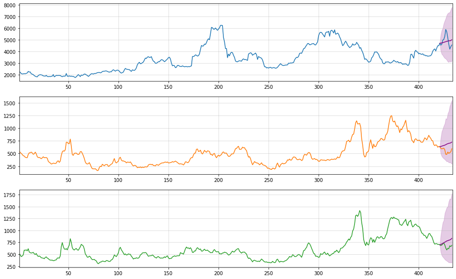
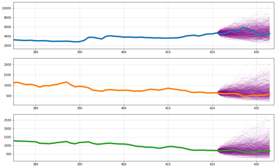
Sample trajectories
fig, ax = plt.subplots(3,1, figsize = (16,10))
for s in range(500):
    [ax[i].plot(np.arange(len(oils)-13,len(oils)),np.concatenate([[oils.iloc[-13,i]],samples_retrans[i][:,s]]), label = "Mean forecast", color = "purple", lw=0.1) for i in range(3)]
[ax[i].plot(oils.values[:,i],label=oils.columns[i],color="C{}".format(i), lw=5) for i in range(3)]
[ax[i].set_xlim((375,len(oils))) for i in range(3)]

[a.grid(alpha=0.5) for a in ax]
Conclusion
This was just a rough collection of ideas on how a Copula-LSTM time-series model could look like. Feel free to contact me for more information.
References
[1] Hochreiter, Sepp; Schmidhuber, Jürgen. Long short-term memory. Neural computation, 1997, 9.8, p. 1735-1780.
[2] Nelsen, Roger B. An introduction to copulas. Springer Science & Business Media, 2007.
Leave a Reply